How to Split Cells in Excel
- Go Ask Debbie
- Aug 21, 2020
- 3 min read
Updated: Oct 3, 2020
This is something I've been asked over and over throughout the years: How do I split cells in Excel?
For Example, Sharon, in HR, years ago told me she had a spreadsheet from the HR system of record that exported employees full names into one column. However, she needed to have the first names and last names in separate columns. Whatever your reason or need, this is actually very simple.
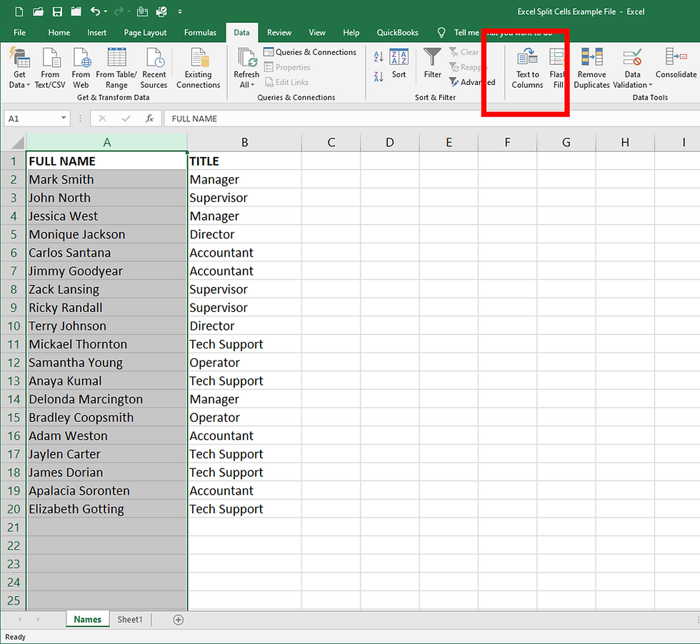
Here's an example of a list of my employees in Excel with the entire Full Name in Column A.

But, Sharon in HR needs to have the First Names in a separate column from the last names.
So, we can do that very easily with the newer versions of Excel (I believe since 2003).
Simply highlight Column A and click on the Data Tab.

On the Data Tab, select "Text to Columns" to start the process.

The Wizard will open, walking you the various options.

Since the current data in Column A lists the First Name, then a Space, and then the Last Name, we will select the "Delimited" option, which happens to be the default.
This means there is something separating (a delimiter or boundary) our data that Excel will be able to recognize in order to split the data into separate columns.
Select the NEXT button and the following page opens asking you various questions about the data.

The default delimiter (separator) is "Tab," but in our case, there is a space between the First and Last Names, so we want to select "Space" as our Delimiter.

Notice in the Data preview section that Excel recognized the space in our data and shows us how it will be separating the data. In this case, it appears that the Last Name now has the Column Header of "Name" because that was the text after the space in the first or header row. We'll just keep it as we know what it is at this point.
You can scroll thru the list, especially if your list is large, to make sure there are no oddities that may not make this separator work for your data.
If the data appears to be separating how you'd like, click the NEXT button.
The next Wizard screen is asking you where you'd like to place the new data - the destination.

By default, Excel will start with the existing column and place the data, in this example, in Columns A & B. However, if your list already has other data in that column, in our example, Column B has the employee's title, then it would replace that data - if you do this accidentally, Excel will tell you and give you a chance to cancel.
But, we're going to be careful and look at the destination placement.
In our case, we can choose Cell C1.
To do this, you can either type it into the Destination field or click into the field and click into your spreadsheet onto the field you'd like the data to start placing your newly separated data. Again, in our case, Cell C1.
Click FINISH on the Wizard and you will now see your split cells or split data in the new cells. In our example, First Names appear in Column C and the Last Names appear in Column D.

Now that your data is separated (or split or delimited, depending on whichever word you use), you can now sort, filter, or do whatever else you need to do with the data now that First and Last Names are in separate columns.
It's that easy!


Comments